
| MANAGEMENT OF
CONVEYANCE |
|
The term conveyance refers to the amount of flow a channel can carry with a given energy slope; it represents the frictional controls imposed on discharge rate by channel cross-sectional shape and roughness.
Bed and bank stabilization treatments can modify cross-sectional shape,
influence roughness, and otherwise influence channel conveyance. The incorporation
of vegetation and LWD into channel and bank stabilization measures frequently
results in rougher channel boundaries than more traditional measures. For
example, plantings of woody vegetation may provide more flow resistance
than riprap revetment. Changes in conveyance properties of a channel can
have both engineering and ecological implications. If flooding or upstream
drainage is an issue at the site in question, the engineer may have to
estimate the impact of proposed measures on flood stages. During low flow
periods conveyance properties affect both depth and velocity which have
important implications for fish and other stream dwelling organisms (see
Special Topic: Physical
Aquatic Habitat). In either case, an environmentally-sensitive
approach to channel protection implies a thoughtful review of the consequences
of any large alteration in existing channel conveyance properties.
UNIFORM FLOW EQUATIONS
The oldest and perhaps simplest approach for computing channel conveyance
for steady flow conditions involves the use of a uniform flow equation
like the Manning or Chezy equation that contains a coefficient that represents
the combined effect of all of the channel characteristics that contribute
to flow resistance. For example, the coefficient n in
the Manning equation:
![]()
reflects channel bed material, bank conditions, planform, and cross-section shape for an entire reach, while Q is the discharge in ft3/s, A is the cross sectional area of the flow in ft2, R is the hydraulic radius in ft, and S is the energy slope. R is equal to A/P, where P is the wetted perimeter in ft, and S is equal to the bed slope when flow is uniform. If SI units are used, the conversion factor in the numerator is simply 1.0 instead of 1.486.
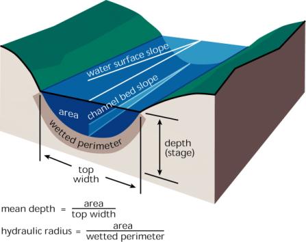 |
Figure
1. Definition of terms in uniform flow equations |
Two other widely used uniform flow formulas are the Chezy formula, which states that
![]()
where C is a flow resistance coefficient, and the Darcy-Weisbach equation
![]()
Where f is a flow resistance coefficient and g is the acceleration of gravity. Both of these formulas are applied using metric (SI) units. Discharge may be computed by multiplying velocity by the cross sectional area: Q = AV.
Regardless of the uniform flow equation used, conveyance
is given by the ratio of discharge, 1 to the square root
of the energy slope, S:K = QS-1/2.
Formulas are available for computing flow resistance coefficients
(n, C and f ) based on the size
of the bed material and the flow depth (Chow 1959, Brownlie
1983). Tables of values are also available in reference
books (e.g., Chow 1959, Henderson, 1966), and photographs
of river channels for which measured n-values are available
are also published in similar works (Barnes, 1967). In
the absence of experience or data, the engineer may examine
these photographs and attempt to match the site in question
to one or more of the photographed sites. Alternatively,
the engineer may assign incremental n-values to each of
about 8 channel characteristics and sum the incremental
values to obtain a composite n for the reach (Cowan, 1956
in Chow, 1959).
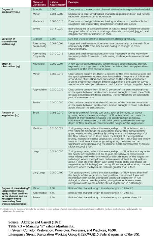
n = (n0 + n1 + n2 + n 3 + n4) m
where:
n0 = base value of n for a straight, uniform, smooth channel in natural materials
n1 = correction for the effect of surface irregularities
n2 = correction for variations in cross section size and shape
n3 = correction for obstructions
n4 = correction for vegetation and flow conditions
m = correction for degree of channel meandering
Appropriate values for these coefficients are provided in Table 1.
TABLE 1: Suggested
values for terms and factors in Cowan equation
for Manning's n |
 |
MANNINGS-N VALUES FOR COMPLEX BOUNDARIES
Channel Bends
One-dimensional flow models do not reproduce
the complex flow phenomena found in channel meander
bends, and the engineer must compensate for this
by increasing the Manning n values for reaches
that are not straight by some factor, as shown
in the Cowan equation above. There are
a variety of semi-empirical techniques for determining
an appropriate value for m, the factor to allow
for meandering in the literature. A review
is provided by James (1994), who tested eight
common techniques using three data sets based
on meandering trapezoidal laboratory channels. One
of the best-performing methods was also one of
the simplest, the linearized SCS method, which
states that
m = 0.43s +
0.57 for s < 1.7
m = 1.30 for s > 1.7
where m is the meandering correction
factor in the Cowan equation above and s is
the channel sinuosity, or the ratio of channel
thalweg length to straight line distance between
the channel endpoints. This method produced
an average absolute error in computed discharge
for a given stage of 8%. This method
produces values in close agreement with the
suggested values for the Cowan equation (e.g.,
Chow 1959). Other methods often show
the dependence of m on the ratio of channel
width to bend radius of curvature, B/rc with
higher values for m for higher values of B/rc.
Composite n Values
Environmentally sensitive channel- and bank-protection
measures often feature treatments that create
highly non-uniform channel boundaries. For
example, large stone may be used along the
bank toe, with woody vegetation on the middle
and upper bank. In addition, complicated
cross-sectional shapes are common, particularly
for high flows (Figure 2). Wide berms
or benches that support various types of vegetation
may occur next to more uniform main channels,
and meander bends in the main channel, floodway
or both are common. In order to use a
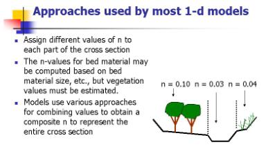
one-dimensional computational model, the engineer
must either compute a single resistance coefficient
for the entire cross-section, or he must subdivide
the cross section into regions of more or less
homogenous flow conditions.
The second approach is discussed below under the heading "conveyance method." Many of the aforementioned computer models have the capability of simulating the effects of irregularly-shaped cross sections with varying types of roughness in different parts of the section using either approach. The models typically contain formulas for combining n-values for different parts of a cross section into a single value, and then the Manning equation shown above is applied to the entire cross section using the "composite" n-value. In order to use such a model to simulate a reach with vegetated boundaries, the engineer must select appropriate n-values for each of the segments ("panels") of the cross section, and when using some models, select an appropriate approach for combining these n-values. Other models provide only one n-composition approach. Information about several composition approaches is summarized in Table 2 below.
 |
Figure
2. Representing a cross section
with varying hydraulic roughness
in a one-dimensional flow model. |
Regardless of the method used to compute composite n-values, the magnitude of the hydraulic influence of vegetation or woody debris is closely related to the fraction of wetted perimeter covered with the vegetation or debris. Clearly, bank vegetation has more influence on the conveyance of narrow channels than wide ones. For example, Masterman and Thorne (1992) presented a case study for a gravel-bed channel with bed material size of 118 mm (4.6 in) and flow depth of 1 m (3.3 ft). For a width/depth ratio of 5, addition of dense vegetation to banks reduced discharge capacity by 38%, but for width/depth ratios of 20 and 30, discharge capacity was reduced only 8% and 6%, respectively.
TABLE
2: Formulas for computing
composite Manning n values,
nc. A=
cross-sectional area, P = wetted
perimeter, R = hydraulic radius
and R = A/P. The subscript i refers
to the ith panel in
the cross section. Panels
are line segments between coordinate
points. |
Method |
Formula
for nc |
Works
well when |
Total
force |
 |
Floodplain
flow depth is more than 30% of
main channel flow depth |
Equal
velocity (used by HEC-RAS for
n variation within the main channel) Chow (1959) |
 |
There
are rough vertical walls or steep
side slopes |
Lotter
Motayed and Krishnamurthy (1980) |
 |
Conveyance Method
When the channel consists of a central main channel and a wide overbank, berm or floodplain on one or both sides, the conveyance method is recommended for flow simulation. In the conveyance method, the channel is treated as several parallel channels for flow computation purposes, and results are simply summed (Figure 3). For example, for the channel shown in Figure 3, the total conveyance, Ktotal = Klob + Kch + Krob. SAM uses the conveyance method as another technique for producing composite hydraulic properties, but HEC-RAS uses conveyance computations in the more orthodox fashion--to analyze flow in overbank and main channel areas more or less separately.
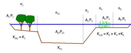 |
Figure
3. Representation
of complex cross section
using conveyance approach. Variables
are defined above. |
Shortcomings of These Approaches
Recent research shows that the boundary between slow-moving flow on the floodplain or berm and faster-moving flow in the main channel is the location for considerable turbulence, leading to momentum transfer and energy losses that are not well represented in either the composite-n or in the conveyance approach. However, these losses are likely much smaller than those due to solid boundary-induced shear except for very narrow channels.
SELECTING N-VALUES FOR VEGETATED BOUNDARIES
Clearly, in order to use the methods prescribed above, the engineer must select reliable n-values for vegetated portions of the channel boundary. Different approaches are needed for flexible and rigid vegetation.
Flexible VegetationDarcy f values for parts of the boundary covered with flexible vegetation may be selected using approaches developed by Kouwen (1988), but this approach requires an estimate of the stiffness of the vegetation and local boundary shear stress.
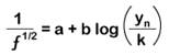
where
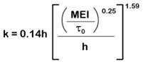
a and b are coefficients that are based on the ratio of total boundary shear , ( t0 = g ynS) to a critical shear for the vegetation, yn is the depth of flow, h is the length of the vegetation, M is the vegetation stem density, E is the modulus of elasticity and I is the stem area’s second moment of inertia. Together, the term MEI represents the overall resistance of the stems to deformation by the flow. Kouwen presents a table of values for a and b that suggest that a and b are equal to 0.15 and 1.85, respectively for erect grasses. The coefficient a varies from 0.20 to 0.29 and b from 2.70 to 3.50 for prone grasses.
Kouwen (1988) suggests that vegetation stiffness may be measured in the field using a simple test that involves dropping a board on the erect grass. He also showed that the results of the board test were highly correlated with grass height for the grasses he tested. For example,
Green grass MEI = 319 h3.3
Dormant grass MEI = 25.4 h2.26
A similar approach for finding n-values for grassed channels was developed by the Soil Conservation Service (1954) that allows selection of n-values based on the type of grass and the product of velocity and hydraulic radius. This technique is included as an option within SAM, but the types and sizes of grass are limited.
Less information is available for flexible woody plants than for grasses. Kouwen and Fathi-Moghadam (2000) present results of tests on four woody coniferous species designed to simulate conditions when nonsubmerged flexible vegetation occurs in vegetated zones of river cross sections. An iterative procedure is again required. The user may read Manning n values from the table below given a flow velocity. Tabulated n-values must be corrected as follows
Corrected n = (tabulated n)[(a/at)(yn/h)]1/2
Where a = total top-view area of the canopy of a typical individual tree or shrub, at = total area of simulated floodplain divided by the number of trees or shrubs, yn = depth of flow, and h = height of vegetation (without deformation due to flow). For example, a floodplain conveying flow 1 m deep at 1.0 m/s supporting 75% cover of cedar trees 2 m high would have a Manning n value ofCorrected n = 0.112*[0.75*(1/2)]1/2 = 0.069
Additional species-specific empirical relationships for Manning values for regions covered by flexible woody vegetation are provided by Copeland (2000), who provides a synthesis of findings for a flume study involving 220 different experiments and 20 shrubby plant species tested over a range of depths and velocities (Freeman et al. 2000). In general, it was found that flow resistance increased with flow depth for partially submerged shrubs and woody plants. However, as flow depth increased, the plants bent and became submerged at flow depths less than 80% of the plant height. Resistance decreased with flow velocity for submerged plants as they bent and presented a more streamlined profile to the flow. The leaf mass or foliage canopy diverted flow beneath the canopy, resulting in significant velocities along the channel bed and general scour. The aforementioned empirical relations are rather complex power-law regression functions.
Rigid Vegetation Including Large Woody
Debris
Manning's n-values for regions covered with
rigid vegetation or woody debris depend upon
the size and spacing of the rigid objects (say,
trees) and whether they are submerged or protrude
through the free surface. Semi-empirical
equations are available that allow computation
of Manning's n given vegetation density and
the drag coefficient. This approach is
illustrated in some detail by Arcement and
Schnieder (1989), but they use an "effective" drag
coefficient based on field data that is about
10 times greater than laboratory measurements. Shields
and Gippel (1995) used a similar approach,
but with drag coefficients based on laboratory
flume data to compute the influence of large
woody debris on Darcy f. Manning
n values for rigid vegetation are highest for
emergent or just-submerged vegetation and decline
as vegetation becomes more deeply submerged
(Shields and Gippel 1995; Wu et al. 1999).
HEC-RAS allows n-variation with stage, but
the user must decide how n depends on stage. As
noted above, flexible vegetation may be flattened
at higher stages, reducing n, and submergence
of low, rigid debris or vegetation also reduces
n. However, flow across a floodplain
may encounter higher n values as stage increases
and flow encounters the crowns of trees.
TABLE 3: Estimated Manning's n for vegetated zone of rivers and floodplains in metric (SI) units from Kouwen and Fathi-Moghadam (2000)
Velocity (m/s) |
Velocity (ft/s) | Cedar |
Spruce |
White pine |
Austrian pine |
0.1 |
0.3 |
0.190 |
0.201 |
0.198 |
0.208 |
0.2 |
0.7 |
0.162 |
0.171 |
0.169 |
0.178 |
0.3 |
1.0 |
0.148 |
0.156 |
0.154 |
0.162 |
0.4 |
1.3 |
0.138 |
0.146 |
0.144 |
0.151 |
0.5 |
1.6 |
0.131 |
0.139 |
0.137 |
0.144 |
0.6 |
2.0 |
0.126 |
0.133 |
0.131 |
0.138 |
0.7 |
2. |
0.122 |
0.129 |
0.127 |
0.133 |
0.8 |
2.6 |
0.118 |
0.125 |
0.123 |
0.129 |
0.9 |
3.0 |
0.115 |
0.121 |
0.120 |
0.126 |
1.0 |
3.3 |
0.112 |
0.118 |
0.117 |
0.123 |
1.1 |
3.6 |
0.110 |
0.116 |
0.114 |
0.120 |
1.2 |
3.9 |
0.107 |
0.114 |
0.112 |
0.118 |
1.3 |
4.3 |
0.105 |
0.111 |
0.110 |
0.115 |
1.4 |
4.6 |
0.104 |
0.110 |
0.108 |
0.113 |
1.5 |
4.9 |
0.102 |
0.108 |
0.106 |
0.120 |
1.6 |
5.2 |
0.101 |
0.106 |
0.105 |
0.110 |
1.7 |
5.6 |
0.099 |
0.105 |
0.103 |
0.109 |
1.8 |
5.9 |
0.098 |
0.103 |
0.102 |
0.107 |
1.9 |
6.2 |
0.097 |
0.102 |
0.101 |
0.106 |
2.0 |
6.6 |
0.096 |
0.101 |
0.100 |
0.105 |
Temporal Factors
When trying to simulate flow effects
of vegetation, the user must decide if seasonal
factors should be considered. Case studies
show that flow resistance due to deciduous
vegetation in full leaf is much greater than
for dormant (winter) conditions (Chow 1959,
Wilson 1973). HEC-RAS allows input of
constant factors for adjusting n-values by
month. Finally, over the long term, vegetation
may impact conveyance by inducing sediment
deposition. Inclusion of sedimentation
in the hydraulic analysis for a project will
increase the cost and complexity of the analysis
several times.
REFERENCES
Aldridge, B.N., & Garrett, J.M. (1973).
Roughness coefficients for stream channels
in Arizona. (U.S. Geological Survey Open-File
Report), 87 pp.
Arcement, George J. Jr., & Schneider,
Verne R. (1989). Guide for selecting Manning's
roughness coefficients for natural channels
and flood plains. (United States Geological
Survey Water-Supply Paper 2339). Denver,
Colorado: United States Government Printing
Office. (pdf)
Barnes, H.H., Jr. (1967). Roughness
characteristics of natural channels. (U.S.
Geological Survey Water-Supply Paper 1849),
213pp. http://www.engr.utk.edu/hydraulics/openchannels/Index.html
Brownlie, W. R. (1983). Flow depth in sand
bed channels. Journal of Hydraulic
Engineering, 109 (7), 959-990.
Brunner, G. W. (2001). HEC-RAS, River Analysis
System User’s Manual. US Army
Corps of Engineers Hydrologic Engineering Center,
Davis, CA (pdf)
Chow, V. T. (1959). Open-channel
hydraulics. McGraw-Hill Book Company,
New York.
Copeland, R. R. (2000). Determination of flow
resistance coefficients due to shrubs and woody
vegetation. Technical Note No. ERCD/CHL
CHETN-VIII-3, U. S. Army Engineer Waterways
Experiment Station, Vicksburg, MS. (pdf)
Cowan, W. L. (1956). Estimating hydraulic roughness
coefficients. Agricultural Engineering.
37(7). 473-475.
Federal Interagency Stream Restoration Working
Group (FISRWG) (1998). Stream Corridor
Restoration: Principles, Processes, and
Practices. GPO Item No. 0120-A;
SuDocs No. A 57.6/2:EN 3/PT.653. ISBN-0-934213-59-3. (pdf)
Freeman, G. E., Rahmeyer, W. H., & Copeland,
R. R. (2000). Determination of resistance due
to shrubs and woody vegetation. (Technical
Report No. ERDC/CHL TR-00-25), U. S. Army Engineer
Waterways Experiment station, Vicksburg, Mississippi,
62pp. (pdf)
Henderson, F. M. (1966). Open-channel flow. New
York, MacMillan Publishing Co., Inc., 522 pp.
James, C. S. (1994). Evaluation of methods
for predicting bend loss in meandering channels.
Journal of Hydraulic Engineering,. 120(2):
245-253.
Kouwen, Nicholas. (1988). Field estimation
of the biomechanical properties of grass. Journal
of Hydraulic Research, 26(5):559-567.
Kouwen, N. & Fathi-Moghadam, M. (2000).
Friction Factors For Coniferous Trees Along
Rivers. Journal of Hydraulic Engineering,
126(10)732-740.
Masterman, R. & Thorne, C. R. (1992). Predicting
Influence of Bank Vegetation on Channel Capacity. Journal
of Hydraulic Engineering, 118(7):1052-1058.
Motayed A. K. & Krishnamurthy, M. (1980).
Composite roughness of natural channels. Journal
of Hydraulic Engineering Division, 106(HY6):1111-1116.
Oplatka, M. (1998). Stablititat von weidenverbauungen
an flussufern. Versuchsanstalt
fur Wasserbau, Hydrologie und Glazioloige der
ETH Zurich. 156, 244.
Shields, F. D., Jr., & Gippel, C. J. (1995). Prediction
of effects of woody debris removal on flow
resistance. Journal of Hydraulic Engineering.
121(4):341-354. (pdf)
Thomas, W. A., Copeland, R. R., Raphelt, N.
K., & McComas, D. N. (1993). User's
Manual for the Hydraulic Design Package for
Channels (SAM) . U.S. Army Corps of Engineers
Waterways Experiment Station, Vicksburg, Mississippi.
USDA (1954). Handbook of channel design
for soil and water conservation. Prepared
by Stillwater Outdoor Hydraulic Lab., Stillwater,
OK., Soil Conservation Service, U.S. Department
of Agriculture, Washington, D.C. (pdf)
Wilson, K. V. (1973). Changes in floodflow
characteristics of a rectified channel caused
by vegetation, Jackson, Mississippi. Journal
of Research of the U.S. Geological Survey.
1(5): 621-625.
Wu, Fu-Chun; Shen, Hsieh Weh, & Chou, Yi-Ju.
(1999). Variation of Roughness Coefficients
for Unsubmerged and Submerged Vegetation. Journal
of Hydraulics 125(9) 934-942.